Friday, January 2nd, 2015
Context adaptive binary arithmetic coding, often abbreviated as CABAC, is an essential part of modern video compression.
It performs lossless compression of a binary data stream without any prior knowledge of the particular characteristics
of the data. These features make it an attractive algorithm for video compression because it is simple, effective,
relatively fast, and requires no prior (or side band) communication between a client and server.
The most well known codecs that leverage CABAC are H.264/AVC and H.265/HEVC. My own codec,
P.264 also leverages a version of CABAC,
and I recall during the early days of P.264 development that there were surprisingly few sturdy resources available for learning more
about the details of this system.
The goal for this article is to provide a gentle introduction to the process, without delving too
deeply into the underlying theory of it. Additional resources for further reading will be linked inline throughout the article.
Also, for those unfamiliar with basic compression concepts, check out
my previous article on compression fundamentals.
Arithmetic coding is the form of entropy coding that is at the heart of CABAC (as well as the final two letters of the acronym).
We'll begin with an introduction to arithmetic coding, and work our way backwards through the acronym to cover each additional
feature of CABAC, including its binary, adaptive and context adaptive properties.
Arithmetic coding leverages the precision range of a numerical value in order to pack information about a sequence of symbols.
Let's walk through a simple example to visually demonstrate this concept.
Assume we have the following alphabet and symbol probabilities:


Let's also assume that we wish to encode the string BBDCA, and that we will use a floating point variable with
infinite precision to accomplish this. Since our variable has infinite precision, we can store infinitely many values
between 0.0 and 1.0 and we can assign a unique value to every possible sequence of symbols (of all lengths).
Quick note: do not be alarmed by this egregious liberty we've taken — although no computer can store values with infinite
precision, we're merely using them to illustrate our process. Later we will see how to restrict this algorithm to fixed point and
limited precision values.
Arithmetic coding describes a specific and straightforward way of assigning all possible sequences of symbols to values within our
range of 0.0 and 1.0. We accomplish this in the following manner, using the probability model of our alphabet.
First, we create what's called a cumulative distribution function, or cdf for short, that accumulates the probability values of
each symbol in our alphabet within a particular range of values between 0.0 and 1.0. For example, the cdf for our current alphabet is the following:

In this case, our A symbol has a probability of 0.2, and so it occupies the range of 0.0 to 0.2 within our cdf. B has a probability of 0.4, so it occupies the range of 0.2 to 0.6, and so on. This process stacks the probabilities of our alphabet wtihin the 0.0 and 1.0 range, and enables us to begin assigning unique values to sequences.
Coding Algorithm
Using our cdf we could trivially code the single symbol sequences A, B, C, or D, by assigning each symbol to a value
within their own range in the cdf. For example, we could assign any value between 0.0 and 0.2 to represent A. Upon decompression, the
decoder would simply compare the input value against the cdf range to decipher the original symbol. So far this isn't particularly useful, but
what if we continued to repeat this process by packing subsequent symbol values within the range of all previously examined symbols of
a sequence? By repeating this process, we would produce a unique sub-range of values for all possible sequences.
This may seem a bit confusing at first, so let's walk through our example. Our goal is to arrive at a unique value, or range of values, within
the range of 0.0 to 1.0, that uniquely identifies our input sequence of symbols. If we can accomplish this, then our decompression process will
be able to reconstruct the original input sequence from this unique computed value.
Returning to our original sequence, BBDCA, we set a high value to 1.0, and a low value to 0.0. These variables identify
our current usable range, which is simply the full range at the start. We encode our first symbol simply by reducing the usable range based
on the symbol's range in the cdf. Thus, our first symbol of B means that we must set high to 0.6, and low to 0.2.
At this point, our encoder could simply output any value within the range of 0.2 and 0.6, and our decoder would be able to uniquely identify
the first symbol as B. Since we're interested in encoding more than just one symbol however, we continue with the process.
Next we encode our subsequent symbol, another B, by mapping our cdf into our current usable range of 0.2 to 0.6. Notice how we overlay
our cdf such that we scale our symbol probabilities to fit.

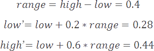
For this second symbol we must again reduce our high and low values to match B's probability range within our current usable range. This results in a high of 0.44 and a low of 0.28. If the encoder now decided to output any value within this range, then the decoder would be able to successfully reconstruct an input sequence of BB.

We repeat this process until we've encoded all symbols in our sequence. Once we're finished, we arrive at a high value of 0.42176 and a low value of 0.4208. If we output any value within this range, then the decoder will be able to successfully reconstruct our entire original input sequence. Common implementations will either output the low value or the midpoint of this range. For our example, we'll output the low value of 0.4208.
Decoding Algorithm
The decoding process is relatively straightforward, and follows from the encoding process. We begin by comparing our coded value of 0.4208
with our cdf. We discover that this value lies within B's range of 0.2 to 0.6, so the first reconstructed value is B.
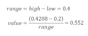
Similar to our encoding process, we now adjust 0.4208 to map inside B's range by subtracting the start of this range
(0.2) and then dividing by the width of this range (0.4). Note that we also maintain high and low values that track our
current usable range.

We then compare this new result against our cdf to determine our second symbol. Since 0.552 falls within our B range of 0.2 to 0.6, we know that our second symbol must be B. We continue this process of mapping values into symbol ranges and then comparing the results against our cdf table in order to reconstruct the full sequence.
Now that we've successfully encoded each symbol in our sequence, there's still one more issue that we need to consider — how will the
decoder know when to finish the reconstruction process?
To better illustrate this question, let's consider the results of encoding the following sequences: A, AA, AAA, and
AAAAAA. Notice that each of these sequences encodes to the exact same value: 0.0. If you experiment with this you will find that,
with our current design, any arithmetically encoded value will be perpetually decoded by the decoompressor. This will result in extra erroneous
symbols being appended onto an output, which prevents us from correctly reconstructing a unique input sequence.
There are two common ways to solve this problem:
We could supply metadata to indicate the number of encoded symbols encoded in the stream. The decoder would then decode the stream and halt once it had processed the specified number of symbols.
Alternatively, we could reserve a special symbol to represent a sentinel symbol. Once the decoder sees this reconstructed symbol it would halt its processing.
What we've just described is known as floating point arithmetic coding. It uses infinite precision to code alphabets and sequences of arbitrary lengths. In practice, for both physical and performance reasons, we must rely upon finite precision and fixed point values, so let's discuss fixed point arithmetic coding.
As noted earlier, floating point coding is impractical for real world computers, so we must implement our arithmetic coder with finite
precision. Additionally, we'll switch over to fixed point values to leverage the integer performance available in many processors,
and to allow us to easily switch between bit depths. We'll use 16 bit values for the remainder of this article, but alternate bit depth
solutions flow trivially from this design.
Fixed point arithmetic coding follows the same general principles of floating point coding but relies on fixed point integers
to store the high, low, and output values. Returning to our original example, our cdf is now:

Similar to our previous walk-through, we begin by setting our high value to 65535, and our low value to 0. We then move along our input sequence and adjust our high and low values based on the probability ranges of each input symbol. After encoding our first symbol, our range is reduced to the following:

So far we've encoded the first symbol in our sequence, a B. Next we encode our second symbol, and our valid range becomes the following:

You may have noticed that we are running out of precision to encode additional symbols. We didn't have this issue with floating point coding because our precision was infinite. With fixed point encoding, we quickly arrive at a valid range that is too small to uniquely encode each symbol's probability range, and so we need to modify our process.
E1, E2, and E3 Scaling
When selecting the fixed point precision of the coder, it is important that sufficient precision is guaranteed so that the entire
cdf can fit within half of the provided precision. For example, if a cdf requires the use of 32,767 distinct values to encode
a single symbol, then the arithmetic coder should use a minimum of 16 bits of precision.
Provided we've used a large enough integer format, then we can employ one of the following three different scaling operations
to prevent us running out of precision while coding a sequence. After each symbol is encoded, we check our current
high and low values, and optionally perform one of the following:
E1 Scaling:
If our high and low values both occupy the lower hemisphere of our full range (i.e. <= 37,767), then this means that all future
values will be fully contained within this lower range. As a result, we can output a 0 to our output stream, and scale our
high and low values back into our full integer range.

The scaling operation is a simple multiplication to double our usable range. This is usually accomplished with a simple shift left operation.

E2 Scaling:
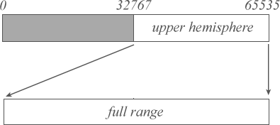
If our high and low values both occupy the upper hemisphere of our full range (i.e. >= 37,768), then this means that all future
values will be fully contained within this upper range. As a result, we can output a 1 to our output stream, and scale our
high and low values back into our full integer range.

E2 scaling first moves our range down to the lower hemisphere, and then performs an e1 scale as follows:

E3 Scaling:
If our high and low values straddle the mid point of our range, causing our values to be within 1/2 precision of each other, then
So far we've guaranteed that our encoding process will always have at least half the full integer precision available if the
high and low values are both contained within the same hemisphere. But what if our values straddle the mid point of our range,
thereby reducing our available precision?
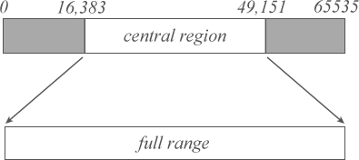
If our low value is greater than one quarter of our range (16,383), and our high value is less than three quarters of our range (49,151),
then we perform an e3 scaling operation to push both values outward.

We accomplish an e3 scaling operation with the following:

We cannot output a 0 or 1 because we do not yet know whether our values will be confined to the upper or lower range. Instead, we'll increment an e3 counter variable that will track the number of consecutive e3 scaling operations performed. The next time we encounter either an e1 or e2 scaling operation, we will reset our e3 counter and do the following:
If e1 scaling, output a 0 and then n 1's, where n equals the e3 counter.
If e2 scaling, output a 1 and then n 0's, where n equals the e3 counter.
After performing a scaling operation, we re-check our newly adjusted high and low values. If the values still require scaling, then we repeat the necessary scaling operation and check the values again. We repeat this process until our high and low values occupy different hemispheres and are at least 1/2 our precision range apart.
Decoding with support for e-scaling is slightly more involved because we need to properly account for the scaling operations that occurred during the encoding phase. Luckily, this process is essentially the inverse of the encode scaling process. After we decode each symbol we check our high and low values. If the criteria for an e-scale has been met, we perform the necessary scaling operation but instead of writing out a 0 or a 1, we shift in the next bit from our input stream.
Binary arithmetic coding (BAC) refers to an arithmetic coder that only operates on alphabets with precisely
two specific symbols: 0 and 1. Binary coders are an attractive solution because they are simple and may be heavily optimized.
Also, since the alphabet of a binary coder is always known, no additional communication is necessary between an encoder and decoder in
order to define and agree on the set of symbols in an alphabet. For these reasons, binary coders are also particularly useful for adaptive
coding (which we'll get to in a moment).
The biggest drawback to binary arithmetic coders is that they are unable to take advantage of higher level structural similarities
in a sequence. Let's use the following example to illustrate this important point.
Assume we have the binary sequence 001011010010010 and wish to analyze the minimum coding rates when using a binary model versus a multi-symbol model.
Binary Model:
If we use a binary model, then our sequence consists of 15 symbols with 9 zeroes and 6 ones. Assuming that our input string is
representative of our probability model, we compute the Shannon entropy of this model to be 0.97 bits per symbol.
We then multiply our entropy by the number of symbols in the input to realize a minimum compressed size of 15 bits
for this sequence.
Multi-Symbol Model:
If we use a multi-symbol model, then our sequence consists of 5 symbols: 1x 001, 1x 011, and 3x 010. We compute the entropy of this model
to be 1.37 bits per symbol. If we multiply this value by the number of symbols in our sequence, we arrive at a total minimum
compressed size of 7 bits.
We can clearly see that a multi-symbol processor could potentially produce a more efficient result. The insight here is that, by combining binary values into higher level symbols, we are reducing the number of symbols in our sequence at a faster rate than the increase in entropy. Furthermore, since our model does not include all combinations of three digit binary symbols, we might be able to gain even further efficiencies.
The operation of a binary coder is almost identical to that of the fixed arithmetic coder described in the previous section. The
primary distinction is that instead of a multi-symbol cumulative distribution function, binary coders have a simple two symbol cdf which
can be described by a single value, the mid point. The mid point partitions the probability range into two distinct regions that define
the probabilities for each of the two symbols in the alphabet.
All other operations follow the design of our fixed point arithmetic coding scheme.
Now that we've defined a fixed point binary arithmetic coding scheme, we're ready to make it adaptive. As previously
discussed, one of the advantages of binary coding is that the alphabet is always known and does not need to be communicated between
the encoder and decoder.
This is great, but it leaves out one other necessary piece — the probability model. Without the model,
we do not know which symbol is more common, and this will make it difficult to efficiently encode a sequence.
Adaptive coding is the process of learning a probability model as we code a sequence or sequences. We assume that past symbols in a
sequence are a relatively useful indicator of future symbols, and that the more symbols we process, the more accurate our model
will become.
Adaptive Process
We begin by initializing our cdf to assign equal probability to each symbol:

Then, we begin our regular binary arithmetic coding process, but after each symbol is encoded we update our probability model. If we
encode a 0, we increase the probability of 0's, and similarily if we encode a 1 we will increase the probability of 1's.
For example, if we encode the sequence 00000000, we will arrive at the following cdf that expects a significantly increased probability
of future 0's, and a decreased probability of 1's. The closer our future symbols match this expected probability distribution, the
greater our coding efficiency.

The adaptive decode process is identical to the encode process, and it will learn the exact same probability cdf as it decodes
each symbol. Both processes must have identical cdfs for each iteration in order to ensure proper reconstruction of the input sequence.
The benefits of adaptive binary arithmetic coding are its simplicity, performance (the cdf may be updated very quickly), and the fact that
no side band data needs to be communicated in order to synchronize the encoder and decoder. A significant drawback however is that the
cdf may contain inaccurate data due to abrupt changes in the symbol stream — recall that our adaptive cdf is based on past history and
this history may be significantly different than future symbols. In this case, we need a slightly augmented form of adaptive coding known as
context adaptive arithmetic coding.
As previously described, there are cases where our simple adaptive model will fail to yield efficient results due to
abrupt, or at least historically divergent, changes in the sequence. When this happens, our adaptive model will see significantly
reduced efficiency but it will recover over time.
To speed the recovery of our adaptive cdf, we introduce the notion of contexts which are essentially cached snapshots (or bins) of our
cdf. Only a single bin may be active at a time, and it will specify our current probability model.

After each symbol is coded, we examine the set of recently processed symbols and decide whether to continue using
the current context, or switch to another one.
While a context is active, it's probabilities are updated in the same manner as our adaptive binary coder (described in the
previous section). This gives us the ability to adapt to large or global probability changes, while maintaining our
ability to adapt to more gradual, or local changes.
Contexts should be carefully chosen and modelled after the expected characteristics of the input data. For example, we could
craft our contexts to enable us to quickly adapt to sudden silence in an audio stream, or a sharp transition in a video.
The purpose of this article was to provide a relatively comprehensive summary of the theories and practical considerations of CABAC.
If you're interested in learning more about this form of compression, check out this paper
which describes the design of the CABAC module within the H.264 video codec.
Also, check out this github repo for an example implementation.
Thanks for reading!