Friday, October 23rd, 2015
Over the last decade we've witnessed a transformation in human
interfaces brought on largely by advances in machine learning. Automated phone assistants, voice and text translators, self driving
cars, and much more, are all reliant on various forms of machine learning.
The randomized decision forest is a machine learning algorithm
that's useful for these kinds of tasks. This algorithm gained significant popularity over the last several years and serves as the heart
of the tracking algorithm within the Microsoft's Kinect product.
This article presents a casual introduction to randomized decision forests, follows with a simple example to highlight the
process, and lastly discusses important development considerations. This will not be a rigorous discussion and is intended
for those with a general interest in the subject without any prior experience.
Similar to other machine learning algorithms, the randomized decision forest (RDF) process is composed of two phases: training and classification.
Training is the pre-process that's used to teach the AI how to recognize particular patterns in a data stream. Classification is the process of
asking the AI to recognize new data, according to the rules that were learned during training. Although we will talk about training as a discrete
pre-process, it's useful to note that training can occur continuously and concurrently with classification.
Structurally, a decision forest is a collection of binary decision trees that have been trained and configured to detect similar features.
We train these trees by exposing them to sample data that is paired with ground truth information. What makes a forest a randomized forest
is that each of its constituent trees is trained using a different subset of the total available training data.
To demonstrate the training process, let's assume that we wish to teach a very smart rabbit how to recognize a soccer (or fútbol) ball. We train the rabbit
by showing it a series of spherical objects, and identify for it the ones that are soccer balls (through some primitive method of communication). In this
case the spherical objects comprise our training data set, and the identification of each object (soccer ball or not) is our ground truth.
Of course, if the rabbit understood human language then we could teach it simply by verbally describing a soccer ball, but that's an analogy for another area of artificial intelligence (see natural language understanding).
Over time, as we assist the rabbit in identifying more and more objects, it will become better at classifying soccer balls. The rabbit will implicitly learn the shape, size,
and color of a soccer ball, while also learning the qualities that disqualify an object. This process is called supervised learning, because we are supplying ground truth
information.
If our algorithm was designed to recognize patterns and generate inferences from data without the use of ground truth information during training, then it would be an unsupervised learning algorithm. Similarly, a semi-supervised algorithm is one that trains on a data set with only partial ground truth information.
It's our job to show the rabbit as many different kinds of soccer balls as possible in order to best enable it to properly classify a new object that it has never seen before.
To offer a sense of the necessary scale, consider that one of the Microsoft Kinect training data sets
consists of almost 720k frames of data.
We can also see from this example that the rabbit is highly dependent upon the quality of the ground truth information. If noise were introduced into the ground truth it would distort
the rabbit's training and ability to correctly classify soccer balls. A smaller amount of accurate training data can be equally as effective as a larger amount of noisy data.
With this analogy in mind, let's start discussing the technical details of this process. As mentioned, this process is divided into two phases: training and classification.
The training phase is responsible for producing the set of decision trees that comprise our forest. We will train each tree using a different subset of our total training data
in order to reduce the overall variance of our forest.
To understand this point better, assume for a moment that we used only a single tree in our forest, and that it was trained using the entire training set. This solitary tree will
be overfitted to the training set, including any potential noise in the data. This will increase the chances of misclassification, and reduce the effectiveness of our system. To
cope with this, we train multiple trees using different subsets of our total data. Each tree will be different, but by using their consensus during classification we can improve
our overall accuracy for the forest.
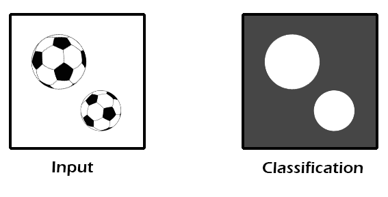
Keeping with our soccer ball analogy, let us assume that our training data consists of a large number of images of soccer balls and other spherical objects. Each of these images is paired with a ground truth image that identifies, for each pixel in the image, whether the pixel belongs to a soccer ball or not. In the figure below, we identify soccer ball pixels in the ground truth as white, and non-soccer-ball pixels as dark gray.
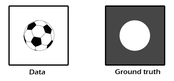
Example training image with ground truth. The ground truth image identifies soccer ball pixels as white, and non-soccer-ball pixels as dark gray.
We've arbitrarily decided to have five binary trees in our forest, and that each tree shall have a depth of no greater than ten. The process of building each tree is the
same, and follows these steps:
Step One: Design our decision function.
Our decision function is responsible for sorting pixels into one of two buckets (left and right). The goal of the decision function is to separate soccer ball pixels from
non-soccer-ball ones, but it's ability is limited, and it is only weakly correlated with the true classification. We call these classifiers weak learners, and they are the
heart of each node in the decision tree.
The following is a basic pseudo-outline of a decision function. It simply accepts a sample from the training set as well as a set of heuristic variables, and returns a value
indicating whether the sample should be sent to the left or right child of the current node.
bool decision_function(sample s, offset, operation) {
  color a = color of sample s;
  color b = color of sample (s + offset);
  return a operation b;
}
Our decision function compares two samples from the training set, and returns true (left) or false (right) based on the color values of each sample. When constructing our trees,
we will randomly and repeatedly select values for our heuristic parameters to refine the accuracy of each decision node.
Step Two: Select a subset of the training data.
We train each tree using a subset of the total training data. Each subset should be large enough to effectively represent the data, but not so large that it encourages
similarities among our trees.
For our example we will select a random sample of 90% of the total training data. Each tree will have a high degree of overlap in its
training set, but will be distinct enough to effectively reduce the overall variance of our forest.
Step Three: Construct our forest.
We are now ready to build our forest, one tree at a time, and one tree decision node at a time. We start by constructing the root node for our first tree, and use a similar
process for each additional node. We want to determine the best set of heuristic parameters for our node, and we derive them heuristically through the following process:
Configure our parameters at random: we select a random offset and operation. Our offset will be chosen within a fixed boundary based on the maximum soccer ball image size that we wish to classify. For this example we will always use an operation of less than, so that we will return left if a is less than b and right otherwise.
Process every pixel in every image in our input training data set using our decision function and parameters, and collect the sorted pixels into left and right pixel buckets.
Analyze the effectiveness of the sorting operation, and keep track of a best candidate. To accomplish this we calculate the entropy of the sorted pixels and determine the information gain of the function.
Entropy is a measurement of the chaos or disorganization within a data set. We can use this principle to measure the effectiveness of our decision function.
We will compare the
entropy of the incoming pixel data (from a parent node bucket) with the entropy of the left and right buckets. If our sorting process has improved the organization of the data,
then it has at least partially managed to separate soccer ball pixels from non-soccer-ball ones.
Entropy is computed using the following formula:
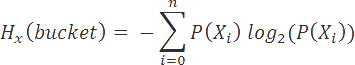
In our case, we have only two types of pixels, soccerball or not, so our vector X simply contains these two types. P(Xi) is the probability
of a given pixel type in the data set. Thus, P(soccerball) is computed by dividing the number of soccerball pixels in the set, by the total number of pixels in the bucket.
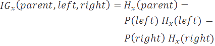
We compute the information gain as the difference between the entropy of the parent and the weighted entropies of the children. This tells us how much better organized
the data has become, as a result of our candidate decision function.
We repeat steps a through c many (e.g. 1,000+) times and select the best heuristic parameters that we find.
At this point we've derived a root node that contains a single decision function plus a set of heuristic parameters. This is the best decision node we found within the
constraints of a simple decision function and a limited number of trial iterations.
Nevertheless, this node manages to divide the total input set of pixels into two
groups with a reduced total entropy.
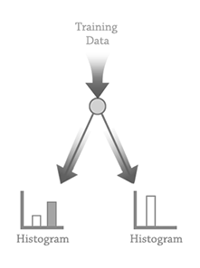
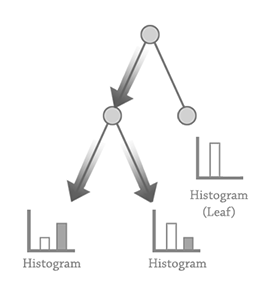
The diagram above depicts this initial process. Training data is fed into a decision function for the root node, and two buckets of pixels are collected. The histogram of each output helps us measure the effectiveness of the decision parameters.
We now repeat this full process to generate left and right child nodes of our root. Each child node operates on the respective bucket produced during the root node
construction.
Note that, depending upon the architecture, we may simply cache the left and right bucket contents from the best node candidate so that we can pass these
as inputs into the left and right node construction processes.
We repeat this process but halt the expansion of a node if one of the following conditions is reached:
We reach our maximum depth (10, in our case).
Entropy reaches zero (or some threshold).
We fail to find a decision function that reduces entropy.
Once any of these conditions is met, we've arrived at a leaf node of our decision tree. This node is simply responsible for recording a histogram of the incoming pixel data. If a large majority of the pixels reaching this node are soccer balls, then we say that this node presents a strong confidence in its classification.
Tree depth and entropy
Whenever our entropy threshold is reached (the data has become sufficiently organized), we halt processing of the current path, and store the results as a leaf node.
In the ideal case, all of our leafnodes contain an entropy of zero, and the data is perfectly sorted.
Unfortunately, this is unlikely to happen for complex data sets, and we may reach a leaf node with a relatively high level of entropy. This implies that
the tree was unable to effectively sort the data and we should consider increasing the maximum tree depth, changing our decision function, revising our training
data set, or leveraging a different algorithm entirely.
Step Four: Repeat steps 2 and 3 four additional times, to generate all five trees for our forest.
This completes the process for building our randomized decision forest. We save the decision trees out to disk (including their decision function parameters and leaf node histograms).
Training can take a very long time, but luckily classification is quick.
Classification is where we start to make practical use of our randomized decision forest. With the training process completed, we will classify a new image that may contain a
soccer ball, by processing each of its pixels using our decision forest.
For each pixel in the image we perform the following:
for each tree t in our forest
  beginning with the root node n of tree t,
    execute n's decision function
      if the result of the decision is left, traverse left
	  if the result of the decision is right, traverse right
    repeat until a leaf node is reached
      record the leaf node classification histogram
After completing this process for each of our five trees, we will have five histograms for every pixel in our image. We average these histograms in order to
obtain a variance reduced histogram. We select the highest probability classification for each pixel, and store it in a classification image.
The final result is this classification image that tells us what the decision forest thinks it sees at each pixel (with the highest confidence). The
following figure shows us a new image of a soccerball that we can classify with our forest on the left. On the right we see an image that resembles a ground truth image, but
is actually an output classification image produced by our forest for the input image. We've color coded each pixel based on the classification value with the highest probability
in each pixel's histogram.
Source image (left) and resultant classification output (right). White classification values identify soccerball pixels, while dark gray indicates a non-soccerball pixel.
Imagine if we selected a specific pixel within our final output image and wanted to visualize the decisions that arrived at this classification. We can accomplish this by walking down the path of each tree and recording the pixel offsets that were used by each decision function. The following image shows us the pixels that were considered by just one tree in our forest.
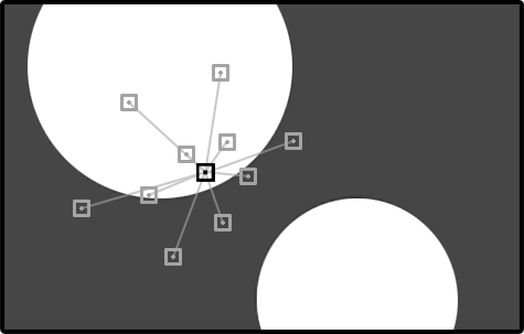
Enlarged classification image focusing on a single tree path for one pixel (in black). The consideration pixel set is highlighted in light gray.
We can see that our black pixel required the consideration of ten neighboring (light gray) pixels in order to arrive at a high confidence classification from one tree. In total, across
all five trees, this decision forest may consider up to 50 neighboring pixels during classification of each output pixel. Note that we've
enlarged the pixel boundaries to make things more visible.
This example focused on training and classification with just two classes of objects: soccer ball and non-soccer-ball. In practice, it's often useful to have several different
classes of objects. We could support this by providing additional ground truth data to help identify additional object types.
One of the biggest issues with randomized decision forests is that the effectiveness of the process is highly dependent upon:
the quality of the decision function
the quality of the training data
the quantity of the training data
As we discuss below, we can partially account for these limitations by adjusting the shape of our decision forest. In some cases however,
we will be unable to overcome these limitations, and alternative machine learning algorithms should be explored. Remember, the randomized
decision forest is simply one machine learning tool in the engineer's belt, and it's important to know when (and when not) to apply it to a problem.
Bias – variance problem
With greater insight into the problem space of the classification we could have perhaps better tailored the operation of the decision function to achieve better results.
During training we randomly selected a tree count of five and a maximum tree depth of ten. If we vary these constraints, we may achieve better results. This brings up an
important point known as the bias-variance problem.
Bias refers to errors caused by improper decisions made by the nodes of our trees, causing us to underfit to our training data. This could cause us to miss important
distinguishing features and lowers our confidence of the classification.
Variance refers to the sensitivity level of our decision functions to detect fluctuations in the training data. A high variance indicates that our tree has overfitted
to the training data and may not recognize important generalized patterns.
It is difficult to balance bias and variance because they are trade offs. Improving one may require worsening the other. We can attempt to cope with bias by deepening our
trees, and we can attempt to cope with variance by increasing the number of trees.
Resource consumption
Our heuristic approach may require us to throw enormous amounts of computing power and memory to train against complicated data sets. There are algorithmic ways of dealing
with these issues, but we can also optimize our process by moving it to the cloud.
To cope with the processing latency of the algorithm we could write both the training and classification phases in CUDA, and execute them on the GPU. For image based
classification, the GPU is particularly well suited to the task, given the highly parallel nature of the algorithm.
To cope with the (generally) large memory requirements of training a large data set, we leverage a distributed MapReduce architecture. Given a controller host machine and a
set of worker machines, we divide the total number of training images amongst the workers and manage the process through the host.
The host selects the decision heuristic parameters and forwards them to each worker machine. The workers are then responsible for processing all of their assigned training
data and reporting back to the host with the classification totals of their respective left and right buckets. The host uses this information to maintain a best candidate
and manage the process of constructing the nodes of the tree. In this manner, no individual machine is responsible for processing the entire input training data, but our
host is still able to make the correct decisions based on the results of the workers.
Hopefully this article has given you a basic understanding of randomized decision forests. If you've enjoyed this material then I would encourage you to investigate other
areas of machine learning, such as convolutional neural networks and recurrent neural networks.
Remember that the randomized decision forest is
a tool that is often used alongside other algorithms in a pipeline, so it's important to understand how its strengths and weaknesses fit within the overall architecture.
Lastly, check out the project page for my
randomized decision forest implementation (source code coming soon).
