Sunday, March 9th, 2014
The knapsack (or backpack) problem is a classic dynamic programming problem. While there are a lot of variations of this problem, this post will only focus on the 0/1 version. This challenge was formally introduced over a century ago and pops up in many different areas including cryptography, resource management, and complexity theory. It is also a popular challenge in programming interviews at several large companies.
(Quick note: for readers who prefer this kind of material in pdf form, grab it here.)
Problem:
Given a backpack that can only hold a maximum weight of W, and a set of n items each with their own weight and value, decide how to most optimally load your backpack. In other words, decide the maximum possible value achievable by packing a subset of items such that the total weight remains ≤ W.
Discussion:
We could solve this with a brute force method by simply enumerating all 2n combinations of items, and selecting the one that best satisfies our criteria.
Alternatively, we could use dynamic programming. The insight here is that, to compute the total weight and value of a set of k (where k ≤ n) items, we actually reuse information about the set of k-1 items. In this way, we can iteratively compute a table v[0...w, 0...n] such that each entry, v[w, i] describes the combined value of the most optimal selection of items (0...i) that is less than or equal to a weight of w. By computing all entries in this table, we will arrive at a solution in cell v[W, n-1].
Let's walk through an example.
Example 1:
Given the items below and a backpack that supports a maximum weight of W=4, compute our maximum achievable value.
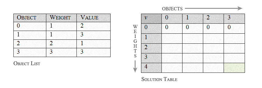
Our object table shows the weight and value of each of our n=4 objects. The solution table represents each of our items along the top row (0...3), and incrementally increasing weights along the first column (0...4).
Each entry in our solution table (v[w,i]) will indicate the maximum value that we can achieve using objects 0...i while remaining less than or equal to a total weight of w. For example, entry v[2,1] will represent the maximum value obtained by selecting some combination of objects 0 and 1 such that the total weight is ≤ 2.
Our final solution cell is highlighted in green, which represents the maximum value achieved when considering all objects and a maximum weight of W=4.
Process:
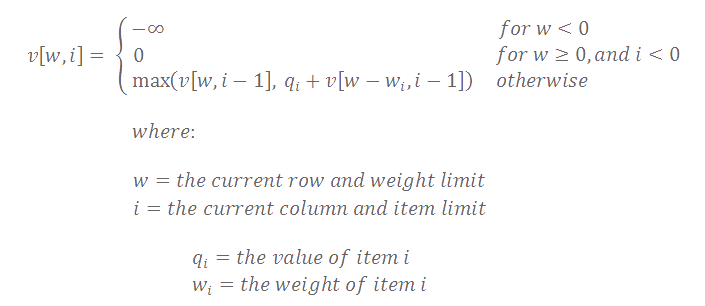
We begin by setting all entries v[0,i] to zero, because a weight of zero will allow us to carry precisely zero objects, and thus result in a zero value. Next we step through the table in row-major order and compute the following for each cell:
Logic:
For each cell, our v[w,i] calculation is making a simple decision for us: do we leave object i or do we take it? Our max operation calculates both options for us, and simply keeps the one that produces the highest value.
Leave object i:
Our first parameter, v[w,i-1], assumes that we should not keep item i, so the value is simply the best we can do with items (0...i-1) and a maximum weight of w. Luckily, we've already calculated this result for cell v[w,i-1], so we simply copy that value.
Take object i:
If we take object i and place it first in our backpack, then we have gained a value of vi but have spent wi in weight. The best we can do now with the remaining objects (0...i-1) and weight w-wi is already computed in v[w-wi,i-1].
Note: if an individual object weight exceeds the allowable weight w, our computation of w-wi will yield a negative value and force our entry v[w-wi,i-1] to equal -∞. When this happens, our max operation will correctly leave the current object.
Filling out our table we arrive at the following:
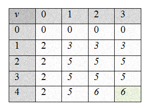
This tells us that the maximum value we can pack into our backpack is 6. Notice that v[4,3] is guaranteed to hold our solution, but it may not be the only valid solution as v[4,2] would also be a valid solution in this particular scenario.
