Friday, January 9th, 2004
A crucial aspect of realistically modelling the interactions between light and participating media is subsurface scattering. This process takes into account the subsurface characteristics of absorbed light, with respect to the microfaceted absorptive and reflective properties of a material. The most recognizable visual result of this process is translucency.
This post describes a very simple technique for simulating the effect of subsurface scattering for use at interactive frame rates inside a game engine. While not a robust solution, if it happens to fit your needs it can be cheap and effective.
Overview
The goal of this technique is to provide a view dependent process for relating the density and material characteristics of an object to approximate how deep a light volume is able to travel through it before being dispersed. This technique is view dependent because it relies upon knowledge of the incident view and lighting angles in order to perform its calculation.
Suppose we have a world composed of a large quad resting on the xz-plane, and a model of a chess piece sitting on top of the quad. We also have a single light source, and a single camera.
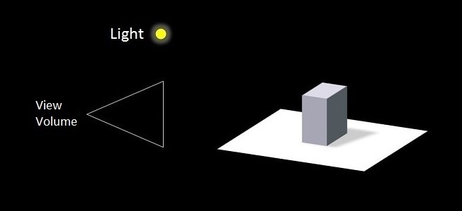
Figure 1: Simple scene arrangement.
We're interested in rendering the chess piece (the parallelepiped in our diagram) such that each pixel is lit according to one of the following conditions:
The pixel is directly lit by the light source
The pixel receives an indirect component due to subsurface light transmission
The pixel is neither directly lit, nor indirectly lit
To achieve this, we perform two additional depth-only passes, from the perspective of the light source, and combine them in a pixel shader during the final scene (color + depth) render. The process is as follows.
Pass One: First Light Pre-pass
The first pass is rendered from the light's perspective, using only the front facing polygons. The output of this pass is a depth map and a normal map. The depth map is used to determine, for each pixel, the location of the nearest fragment to the light source. This information is later used to derive this nearest fragment's visibility to the camera, and ultimately determine which fragments are directy lit, and which are in shadow.
The normal map that we generate in this pass is used to determine the intensity of light arriving at the surface of our object so that we can relate it to the intensity of the light beneath the surface. To generate this map, we output the interpolated normals of the chess piece for every pixel. This is accomplished simply by passing the world space normals to the pixel shader, and writing these values out to the frame buffer. Note that care must be taken to properly convert the normals from normal space to color space.
Pass Two: Second Light Pre-pass
Next we re-render the same frame, but this time we render only the back facing polygons. We cache the output of this path as a second depth map, in the same format and resolution of our depth map generated in the previous pass. By subtracting our front-facing depth map from our back-facing map, we are able to create a very rough estimate of the volume of our chess piece.
The following diagram depicts this process. Imagine a vector traced from the light source into the scene that strikes the chess piece. Fragment a represents the nearest depth coordinate on our chess piece along this vector, while fragment b represents the farthest (note potential caveats here, but we will discuss them later in the article).
By comparing these two depth values we are able to determine how thick the object is, along our particular vector, and we will use this information in a subsequent pass to determine how far light is able to travel through our object at any particular point.
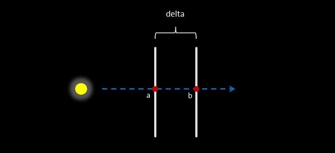
Figure 2: Front facing depth map data is subtracted from back facing data to derive the per pixel thickness of the object.
Pass Three: Final Render Pass
At this point we know the key pieces of information we need to finish this effect:
The orientation of the light source (transform matrix)
The orientation of the viewer (transform matrix)
Front and back facing depth maps of our object
A map of surface normals for our object
Next we render the scene from the viewer's perspective, passing the light and viewer orientation information to the vertex shader. The vertex shader's job is two-fold: it must transform the object vertices from world space into the viewer's clip space (for eventual output for primitive assembly), and it must also transform the world space vertices into the light's clip space (and pass these on to the pixel shader).
The pixel shader is where things get interesting. First we calculate the direct lighting contribution for our (current) fragment. For the purposes of my demo I simply used the Blinn-Phong model.
The next step is to determine whether or not our source fragment is in shadow. We accomplish this by consulting the front-facing depth map. Recall that in our vertex shader we transformed the chess piece's geometry into the light's clip space, which is coincidentally very close to the space in which our depth maps exist. Our goal is to be able to move our light-clip space fragments into the same space as the depth maps, so that we can compare our fragment's depth value to that stored in the front-facing depth map.
Next we must divide the fragment's light-clip-space xyz coordinates by the w coordinate. This accounts for the perspective divide applied to the fragments resulting in the depth values stored in our maps, and effectively moves our coordinates into normalized device space. We must also account for the fact that our depth map is indexed using coordinates ranging from 0 to 1, while our fragment's coordinates range from -1 to 1.
Lastly, we must invert the y coordinate to account for the fact that the depth map is indexed from a <0,0> origin in the upper left, while our fragment's coordinates are based on a 0,0 origin in the lower left. The following pixel shader code performs these transformations:
float pixelViewDepth  = input.objectPos.z / input.objectPos.w;
float2 depthMapCoords = input.objectPos.xy / input.objectPos.w;

depthMapCoords   = depthMapCoords / 2.0 + 0.5;
depthMapCoords.y = 1.0 - depthMapCoords.y;
Now that our coordinates are all in the same space, we can use the fragment's transformed position (xy in light NDC space) as texture coordinates into the front facing depth map. If the value in the texture is less (beyond some epsilon) than our fragment's depth value, then our fragment must be in shadow. Otherwise, we have a directly lit fragment.
If our source fragment is lit directly, we can apply the diffuse and specular values calculated using Blinn-Phong lighting combined with any subsurface illumination contribution. If our fragment is in shadow, then we apply only the subsurface illumination.
The Subsurface Component
The subsurface component is what gives us the effect we're interested in. The first thing we do is trace a line from the light source to our view space fragment coordinate. What we're interested in is the first location where the ray enters the chess piece - which we'll call our "incident fragment." Luckily we can determine this simply by consulting our front facing depth map. The depth value stored at the fragment's xy coordinate tells us the full xyz coordinate (in light NDC space) of our incident fragment. The following diagram depicts this step.
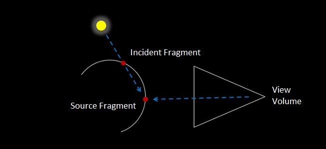
Figure 3: The distance between the source and incident fragments is used to calculate the degree of subsurface illumination at the visible source fragment.
Next we calculate the intensity of the light at the incident fragment location. In order to accomplish this, we need to know the normal at this position. Luckily we extracted this information in a previous pass, and saved it in a texture. By indexing into this texture at the xy coordinates of our incident fragment (which match those of our initial transformed fragment), we can access the normal and perform our lighting calculation.
Using this information, along with the density of the surface and the distance between our source fragment and this incident coordinate, we can approximate the extent to which our source fragment is indirectly lit. We compare our source fragment's light-device space coordinates against the coordinates in both of the depth maps. There are three possibilities for the relative position of our fragment with respect to the light source:
The source fragment is closer to the light than the incident (front facing) fragment
The source fragment is in between the incident (front facing) and back facing fragments
The source fragment is farther from the light source than the back facing fragment
Case (1) implies that the source fragment is directly lit by the light source, and has no subsurface component. Case (2) implies the source fragment is not directly lit (is in shadow), but does potentially receive some subsurface lighting contribution, based on the subsurface distribution function (described in greater detail below). Case (3) implies that the source fragment should receive no direct nor subsurface lighting contributions.
Note an important caveat: if the geometry of the object is sufficiently complex, it may lead to unexpected artifacting. The diagram below highlights one such example. In this case, one may expect an indirect contribution to be applied through the object, and affect fragment c of the same object. Due to the simple nature of this algorithm, light transmission will appear to halt abruptly before reaching point c, despite the intensity of the light source or its proximity to the object. For most cases however, this artifact is permissible, as they can often be designed around.
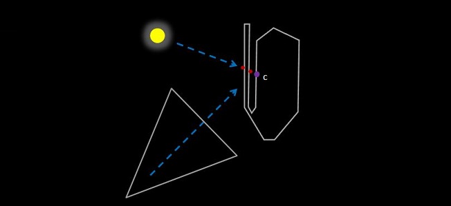
Figure 4: Potential hazard: light will not penetrate the object as expected, leaving fragment c in shadow without any subsurface contribution.
The first and third cases above are fairly straightforward, as no additional work is needed to finish the fragment. Thus for the remainder of this post we assume that our fragment is in between the two coordinates (case 2) because it is the most interesting case.
Subsurface Scatter Contribution
At this point we know the location of the incident fragment, we know how intensely the incident fragment is lit, and we know the location of our source fragment. We're almost ready to plug this information into our energy transfer function and determine whether the fragment should exhibit any degree of translucency. Before we do this however, we determine the scalar distance that light would need to travel in order to reach our source fragment, assuming a linear path from the incident fragment (See Figure 3), and we calculate this by subtracting the z-depth of our incident fragment from the z coordinate of our transformed (into light space) source fragment.
At long last, we supply the distance that we've derived to our subsurface transfer function. For the purposes of this demo I simply used an inverse square multiplied by a user supplied exponent which can be adjusted to taste. Depending on your needs, this may or may not suffice. An HLSL implementation of my very simple transfer function is as follows:
float3 ssxfer( float distance, float fExp )
{
	return 1.0 / (distance * distance * fExp);
}
Note that values are only supplied to this function if the fragment is legitimately qualified to receive a subsurface component. If appropriate, the result of this transfer function may then be added to a direct illumination component. The following screenshots demonstrate the results of this transfer function applied to our demo scene.
Final Results
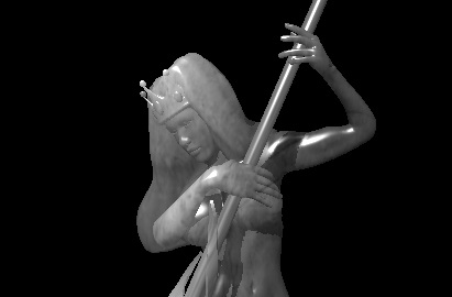

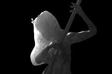
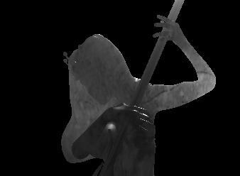
Conclusion
In the end this is a very simple algorithm which is merely an extension of traditional shadow mapping. The results are useful in creating an inexact and physically incorrect visual approximation of the perimeter translucency effect caused by subsurface scattering. In many cases however, this approximation is sufficient to achieve the impression of a lighting model with true subsurface scattering support.
More Information
For more information, including videos and downloadable versions of this post and software, visit my subsurface scattering approximation project page.
